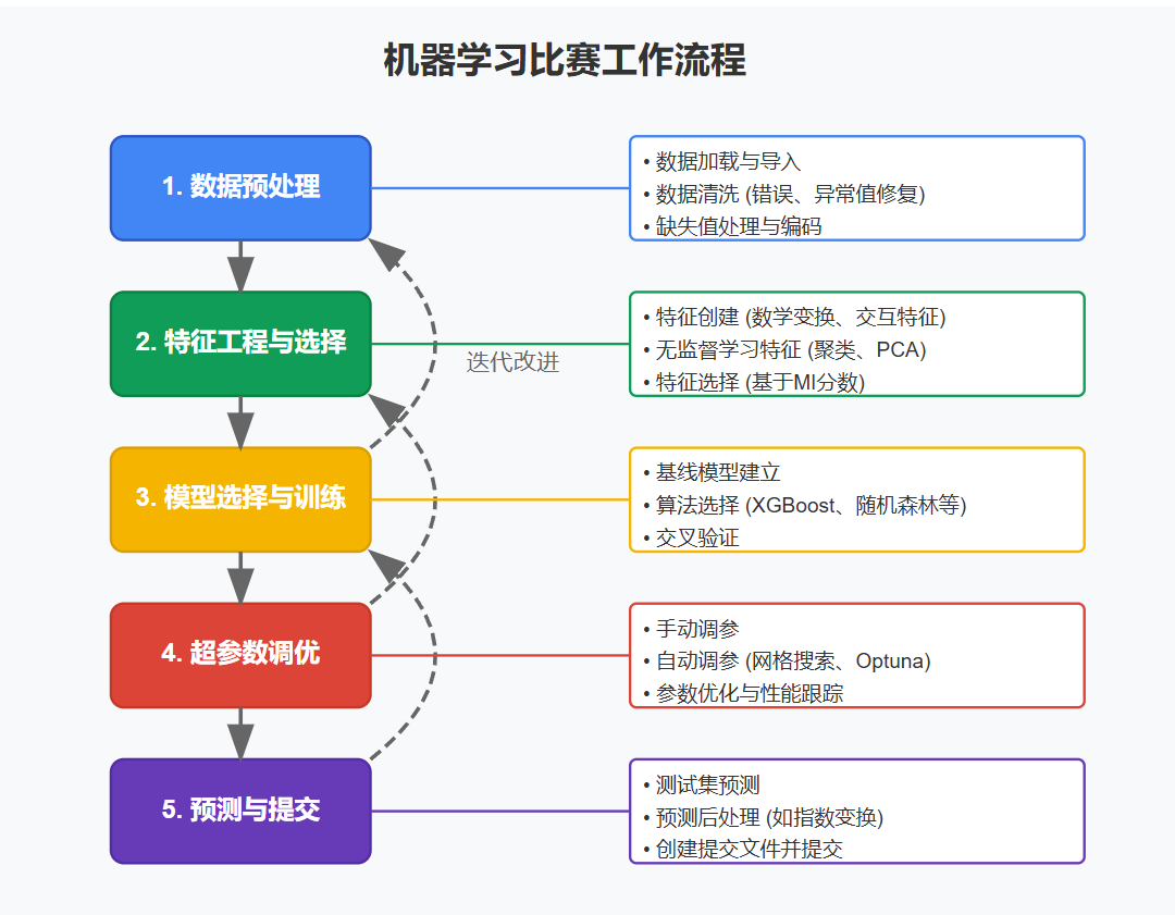
引言

欢迎来到特征工程项目，这个项目是为 House Prices - Advanced Regression Techniques 竞赛准备的！本次竞赛使用的数据与在 [特征工程](Feature Engineering) 课程练习中使用的数据几乎相同。我们将把您之前完成的工作整合成一个完整的项目，您可以在此基础上加入自己的想法。

第一步 - 准备工作

导入和配置

我们首先导入在练习中使用的包，并设置一些笔记本默认值：

import os
import warnings
from pathlib import Path

import matplotlib.pyplot as plt
import numpy as np
import pandas as pd
import seaborn as sns
from IPython.display import display
from pandas.api.types import CategoricalDtype

from category_encoders import MEstimateEncoder
from sklearn.cluster import KMeans
from sklearn.decomposition import PCA
from sklearn.feature_selection import mutual_info_regression
from sklearn.model_selection import KFold, cross_val_score
from xgboost import XGBRegressor


# Set Matplotlib defaults
plt.style.use("seaborn-whitegrid")
plt.rc("figure", autolayout=True)
plt.rc(
    "axes",
    labelweight="bold",
    labelsize="large",
    titleweight="bold",
    titlesize=14,
    titlepad=10,
)

# Mute warnings
warnings.filterwarnings('ignore')

数据预处理

在进行任何特征工程之前，我们需要对数据进行预处理，使其适合分析。我们在课程中使用的数据比竞赛数据简单一些。对于 Ames 竞赛数据集，我们需要：

加载来自CSV文件的数据
清洗数据以修复任何错误或不一致性
编码统计数据类型（数值型、分类型）
填充任何缺失值

我们将把所有这些步骤封装到一个函数中，这样您就可以在需要时轻松获取新的数据框。读取CSV文件后，我们将应用三个预处理步骤：clean、encode 和 impute，然后创建数据分割：一个（df_train）用于训练模型，另一个（df_test）用于生成提交到竞赛排行榜打分的预测。

def load_data():
    # 读取数据
    data_dir = Path("../input/house-prices-advanced-regression-techniques/")
    df_train = pd.read_csv(data_dir / "train.csv", index_col="Id")
    df_test = pd.read_csv(data_dir / "test.csv", index_col="Id")
    # 合并分割，以便我们可以一起处理它们
    df = pd.concat([df_train, df_test])
    # 预处理
    df = clean(df)
    df = encode(df)
    df = impute(df)
    # 重新形成分割
    df_train = df.loc[df_train.index, :]
    df_test = df.loc[df_test.index, :]
    return df_train, df_test

清洗数据

该数据集中的一些分类特征在其类别中有明显的拼写错误：

1
2
3

array(['VinylSd', 'MetalSd', 'Wd Shng', 'HdBoard', 'Plywood', 'Wd Sdng',
       'CmentBd', 'BrkFace', 'Stucco', 'AsbShng', 'Brk Cmn', 'ImStucc',
       'AsphShn', 'Stone', 'Other', 'CBlock'], dtype=object)

将这些与 data_description.txt 比较，我们可以看出需要清洗的内容。我们将在这里处理几个问题，不过您可能希望进一步评估此数据。

def clean(df):
    df["Exterior2nd"] = df["Exterior2nd"].replace({"Brk Cmn": "BrkComm"})
    # GarageYrBlt 的一些值已损坏，因此我们将用房屋建造年份替换它们
    df["GarageYrBlt"] = df["GarageYrBlt"].where(df.GarageYrBlt <= 2010, df.YearBuilt)
    # 以数字开头的名称处理起来很麻烦
    df.rename(columns={
        "1stFlrSF": "FirstFlrSF",
        "2ndFlrSF": "SecondFlrSF",
        "3SsnPorch": "Threeseasonporch",
    }, inplace=True,
    )
    return df

编码统计数据类型

Pandas 有与标准统计类型（数值型、分类型等）对应的 Python 类型。为每个特征编码正确的类型有助于确保每个特征被我们使用的任何函数适当处理，并使我们更容易一致地应用转换。这个单元定义了 encode 函数：

# 数值特征已经被正确编码（连续型使用`float`，离散型使用`int`），
# 但分类特征需要我们自己处理。特别注意，`MSSubClass`特征虽然
# 读取为`int`类型，但实际上是（名义型）分类特征。

# 名义型（无序）分类特征
features_nom = ["MSSubClass", "MSZoning", "Street", "Alley", "LandContour", "LotConfig", "Neighborhood", "Condition1", "Condition2", "BldgType", "HouseStyle", "RoofStyle", "RoofMatl", "Exterior1st", "Exterior2nd", "MasVnrType", "Foundation", "Heating", "CentralAir", "GarageType", "MiscFeature", "SaleType", "SaleCondition"]

# 序数型（有序）分类特征 
# Pandas将类别称为"levels"（级别）
five_levels = ["Po", "Fa", "TA", "Gd", "Ex"]  # 五个级别：差、一般、普通、好、优秀
ten_levels = list(range(10))  # 十个级别：0到9
ordered_levels = {
    "OverallQual": ten_levels,        # 整体质量
    "OverallCond": ten_levels,        # 整体状况
    "ExterQual": five_levels,         # 外部质量
    "ExterCond": five_levels,         # 外部状况
    "BsmtQual": five_levels,          # 地下室质量
    "BsmtCond": five_levels,          # 地下室状况
    "HeatingQC": five_levels,         # 供暖质量
    "KitchenQual": five_levels,       # 厨房质量
    "FireplaceQu": five_levels,       # 壁炉质量
    "GarageQual": five_levels,        # 车库质量
    "GarageCond": five_levels,        # 车库状况
    "PoolQC": five_levels,            # 泳池质量
    "LotShape": ["Reg", "IR1", "IR2", "IR3"],  # 地块形状：规则、稍不规则、中度不规则、高度不规则
    "LandSlope": ["Sev", "Mod", "Gtl"],        # 土地坡度：陡峭、中等、平缓
    "BsmtExposure": ["No", "Mn", "Av", "Gd"],  # 地下室暴露程度：无、最小、平均、好
    "BsmtFinType1": ["Unf", "LwQ", "Rec", "BLQ", "ALQ", "GLQ"],  # 地下室完工类型1
    "BsmtFinType2": ["Unf", "LwQ", "Rec", "BLQ", "ALQ", "GLQ"],  # 地下室完工类型2
    "Functional": ["Sal", "Sev", "Maj1", "Maj2", "Mod", "Min2", "Min1", "Typ"],  # 功能性
    "GarageFinish": ["Unf", "RFn", "Fin"],     # 车库完工情况：未完工、粗糙完工、精细完工
    "PavedDrive": ["N", "P", "Y"],             # 铺装车道：否、部分、是
    "Utilities": ["NoSeWa", "NoSewr", "AllPub"],  # 公用设施：无下水道和水、无下水道、所有公用设施
    "CentralAir": ["N", "Y"],                  # 中央空调：否、是
    "Electrical": ["Mix", "FuseP", "FuseF", "FuseA", "SBrkr"],  # 电气系统类型
    "Fence": ["MnWw", "GdWo", "MnPrv", "GdPrv"],  # 围栏：最小木材围栏、良好木材围栏、最小隐私围栏、良好隐私围栏
}

# 为缺失值添加None级别
ordered_levels = {key: ["None"] + value for key, value in
                  ordered_levels.items()}

def encode(df):
    # 编码名义型分类
    for name in features_nom:
        df[name] = df[name].astype("category")
        # 为缺失值添加None类别
        if "None" not in df[name].cat.categories:
            df[name] = df[name].cat.add_categories("None")
    
    # 编码序数型分类
    for name, levels in ordered_levels.items():
        df[name] = df[name].astype(CategoricalDtype(levels,
                                                    ordered=True))
    return df

处理缺失值

现在处理缺失值将使特征工程更加顺利。我们将用 0 填充缺失的数值，用 "None" 填充缺失的分类值。您可能想尝试其他填充策略。特别是，您可以尝试创建”缺失值”指示器：缺失值被填充时为 1，否则为 0。

def impute(df):
    for name in df.select_dtypes("number"):
        df[name] = df[name].fillna(0)
    for name in df.select_dtypes("category"):
        df[name] = df[name].fillna("None")
    return df

加载数据

现在我们可以调用数据加载器并获取处理后的数据分割：

1	df_train, df_test = load_data()

取消注释并运行此单元格，如果您想查看它们包含的内容。注意 df_test 中 SalePrice 的值缺失（NA 在填充步骤中用0填充）。

# 查看值
#display(df_train)
#display(df_test)

# 显示关于数据类型和缺失值的信息
#display(df_train.info())
#display(df_test.info())

建立基准

最后，让我们建立一个基准分数来评判我们的特征工程。

这是我们在第一课中创建的函数，它将计算特征集的交叉验证 RMSLE 分数。我们使用 XGBoost 作为模型，但您可能想尝试其他模型。

def score_dataset(X, y, model=XGBRegressor()):
    # 分类型特征的标签编码
    #
    # 标签编码对于XGBoost和RandomForest很好，但对于
    # Lasso或Ridge等模型，独热编码会更好。`cat.codes`
    # 属性保存了类别级别。
    for colname in X.select_dtypes(["category"]):
        X[colname] = X[colname].cat.codes
    # 房屋竞赛的评估指标是RMSLE（均方根对数误差）
    log_y = np.log(y)
    score = cross_val_score(
        model, X, log_y, cv=5, scoring="neg_mean_squared_error",
    )
    score = -1 * score.mean()
    score = np.sqrt(score)
    return score

我们可以在想要尝试新特征集时随时重用这个评分函数。我们现在使用处理过的数据（没有额外特征）运行它，获取一个基准分数：

X = df_train.copy()
y = X.pop("SalePrice")

baseline_score = score_dataset(X, y)
print(f"Baseline score: {baseline_score:.5f} RMSLE")

Baseline score: 0.14302 RMSLE

第二步 - MI值筛选

在第2课中，我们了解了如何使用互信息计算特征的效用分数，这可以指示特征的潜在价值。这个隐藏单元定义了我们使用的两个效用函数，make_mi_scores 和 plot_mi_scores：

def make_mi_scores(X, y):
    X = X.copy()
    for colname in X.select_dtypes(["object", "category"]):
        X[colname], _ = X[colname].factorize()
    # 所有离散特征现在应该具有整数数据类型
    discrete_features = [pd.api.types.is_integer_dtype(t) for t in X.dtypes]
    mi_scores = mutual_info_regression(X, y, discrete_features=discrete_features, random_state=0)
    mi_scores = pd.Series(mi_scores, name="MI Scores", index=X.columns)
    mi_scores = mi_scores.sort_values(ascending=False)
    return mi_scores

def plot_mi_scores(scores):
    scores = scores.sort_values(ascending=True)
    width = np.arange(len(scores))
    ticks = list(scores.index)
    plt.barh(width, scores)
    plt.yticks(width, ticks)
    plt.title("Mutual Information Scores")

让我们再次查看我们的特征分数：

X = df_train.copy()
y = X.pop("SalePrice")

mi_scores = make_mi_scores(X, y)
mi_scores

输出[12]:

OverallQual    0.571457
Neighborhood   0.526220
GrLivArea      0.430395
YearBuilt      0.407974
LotArea        0.394468
...
PoolQC         0.000000
MiscFeature    0.000000
MiscVal        0.000000
MoSold         0.000000
YrSold         0.000000
Name: MI Scores, Length: 79, dtype: float64

您可以看到，我们有许多信息量很高的特征，也有一些完全不具信息性的特征（至少就它们自身而言）。正如我们在教程2中讨论的，在特征开发过程中，得分最高的特征通常会带来最大收益，因此集中精力在这些特征上可能是个好主意。另一方面，在非信息性特征上训练可能导致过拟合。因此，我们将完全舍弃得分为0.0的特征：

1 2	def drop_uninformative(df, mi_scores): return df.loc[:, mi_scores > 0.0]

移除这些特征会带来小幅的性能提升：

X = df_train.copy()
y = X.pop("SalePrice")
X = drop_uninformative(X, mi_scores)

score_dataset(X, y)

输出[14]:

1	0.14274827027030276

稍后，我们将把 drop_uninformative 函数添加到我们的特征创建管道中。

第三步 - 创建特征

现在我们将开始开发我们的特征集。

为了使我们的特征工程工作流程更加模块化，我们将定义一个函数，该函数接受一个准备好的数据框并通过一系列转换传递它，以获得最终的特征集。它将类似于这样：

def create_features(df):
    X = df.copy()
    y = X.pop("SalePrice")
    X = X.join(create_features_1(X))
    X = X.join(create_features_2(X))
    X = X.join(create_features_3(X))
    # ...
    return X

让我们继续定义一个转换，即对分类特征进行标签编码：

def label_encode(df):
    X = df.copy()
    for colname in X.select_dtypes(["category"]):
        X[colname] = X[colname].cat.codes
    return X

对于使用像XGBoost这样的树集成模型时，对任何类型的分类特征进行标签编码都是可以的，即使是无序类别。如果您想尝试线性回归模型（在这个竞赛中也很流行），您会希望使用独热编码，特别是对于具有无序类别的特征。

使用Pandas创建特征

这个单元重现了您在练习3中完成的工作，您在其中应用了在Pandas中创建特征的策略。修改或添加这些函数以尝试其他特征组合。

def mathematical_transforms(df):
    X = pd.DataFrame()  # 保存新特征的数据框
    X["LivLotRatio"] = df.GrLivArea / df.LotArea
    X["Spaciousness"] = (df.FirstFlrSF + df.SecondFlrSF) / df.TotRmsAbvGrd
    # 这个特征最终没有提高性能
    # X["TotalOutsideSF"] = \
    #     df.WoodDeckSF + df.OpenPorchSF + df.EnclosedPorch + \
    #     df.Threeseasonporch + df.ScreenPorch
    return X

def interactions(df):
    X = pd.get_dummies(df.BldgType, prefix="Bldg")
    X = X.mul(df.GrLivArea, axis=0)
    return X

def break_down(df):
    X = pd.DataFrame()
    X["MSClass"] = df.MSSubClass.str.split("_", n=1, expand=True)[0]
    return X

def group_transforms(df):
    X = pd.DataFrame()
    X["MedNhbdArea"] = df.groupby("Neighborhood")["GrLivArea"].transform("median")
    return X

这里是一些您可以探索的其他转换想法：

质量 Qual 和条件 Cond 特征之间的交互。例如，OverallQual 是一个得分很高的特征。您可以尝试将其与 OverallCond 结合，方法是将两者转换为整数类型并取乘积。
面积特征的平方根。这将把平方英尺的单位转换为简单的英尺。
数值特征的对数。如果特征分布有偏，应用对数可以帮助使其正态化。
描述相同事物的数值和分类特征之间的交互。例如，您可以查看 BsmtQual 和 TotalBsmtSF 之间的交互。
Neighboorhood 中的其他组统计。我们计算了 GrLivArea 的中位数。查看 mean、std 或 count 可能也很有趣。您还可以尝试将组统计与其他特征结合。也许 GrLivArea 与中位数之间的差异很重要？

k-均值聚类

我们用于创建特征的第一个无监督算法是k-means聚类。我们看到您可以使用聚类标签作为特征（一个包含 0、1、2、…的列）或使用观测到每个聚类的距离。我们看到这些特征有时能有效解开复杂的空间关系。

cluster_features = [
    "LotArea",
    "TotalBsmtSF",
    "FirstFlrSF",
    "SecondFlrSF",
    "GrLivArea",
]

def cluster_labels(df, features, n_clusters=20):
    X = df.copy()
    X_scaled = X.loc[:, features]
    X_scaled = (X_scaled - X_scaled.mean(axis=0)) / X_scaled.std(axis=0)
    kmeans = KMeans(n_clusters=n_clusters, n_init=50, random_state=0)
    X_new = pd.DataFrame()
    X_new["Cluster"] = kmeans.fit_predict(X_scaled)
    return X_new

def cluster_distance(df, features, n_clusters=20):
    X = df.copy()
    X_scaled = X.loc[:, features]
    X_scaled = (X_scaled - X_scaled.mean(axis=0)) / X_scaled.std(axis=0)
    kmeans = KMeans(n_clusters=20, n_init=50, random_state=0)
    X_cd = kmeans.fit_transform(X_scaled)
    # 标记特征并加入数据集
    X_cd = pd.DataFrame(
        X_cd, columns=[f"Centroid_{i}" for i in range(X_cd.shape[1])]
    )
    return X_cd

主成分分析

PCA是我们用于特征创建的第二个无监督模型。我们看到它如何被用于分解数据中的变异结构。PCA算法给我们提供了载荷，描述了每个变异成分，也提供了成分，即转换后的数据点。载荷可以暗示要创建的特征，而成分我们可以直接用作特征。

以下是PCA课程中的工具函数：

def apply_pca(X, standardize=True):
    # 标准化
    if standardize:
        X = (X - X.mean(axis=0)) / X.std(axis=0)
    # 创建主成分
    pca = PCA()
    X_pca = pca.fit_transform(X)
    # 转换为数据框
    component_names = [f"PC{i+1}" for i in range(X_pca.shape[1])]
    X_pca = pd.DataFrame(X_pca, columns=component_names)
    # 创建载荷
    loadings = pd.DataFrame(
        pca.components_.T,  # 转置载荷矩阵
        columns=component_names,  # 列为主成分
        index=X.columns,  # 行为原始特征
    )
    return pca, X_pca, loadings

def plot_variance(pca, width=8, dpi=100):
    # 创建图形
    fig, axs = plt.subplots(1, 2)
    n = pca.n_components_
    grid = np.arange(1, n + 1)
    # 解释方差
    evr = pca.explained_variance_ratio_
    axs[0].bar(grid, evr)
    axs[0].set(
        xlabel="Component", title="% Explained Variance", ylim=(0.0, 1.0)
    )
    # 累积方差
    cv = np.cumsum(evr)
    axs[1].plot(np.r_[0, grid], np.r_[0, cv], "o-")
    axs[1].set(
        xlabel="Component", title="% Cumulative Variance", ylim=(0.0, 1.0)
    )
    # 设置图形
    fig.set(figwidth=8, dpi=100)
    return axs

以下是根据练习5产生特征的转换。如果您得出了不同的答案，可能需要修改这些。

def pca_inspired(df):
    X = pd.DataFrame()
    X["Feature1"] = df.GrLivArea + df.TotalBsmtSF
    X["Feature2"] = df.YearRemodAdd * df.TotalBsmtSF
    return X

def pca_components(df, features):
    X = df.loc[:, features]
    _, X_pca, _ = apply_pca(X)
    return X_pca

pca_features = [
    "GarageArea",
    "YearRemodAdd",
    "TotalBsmtSF",
    "GrLivArea",
]

这些只是使用主成分的几种方式。您也可以尝试使用一个或多个成分进行聚类。需要注意的一点是，PCA不会改变点之间的距离 – 它只是一种旋转。所以使用全部成分集进行聚类与使用原始特征进行聚类相同。相反，选择一些成分子集，也许是那些具有最大方差或最高MI分数的成分。

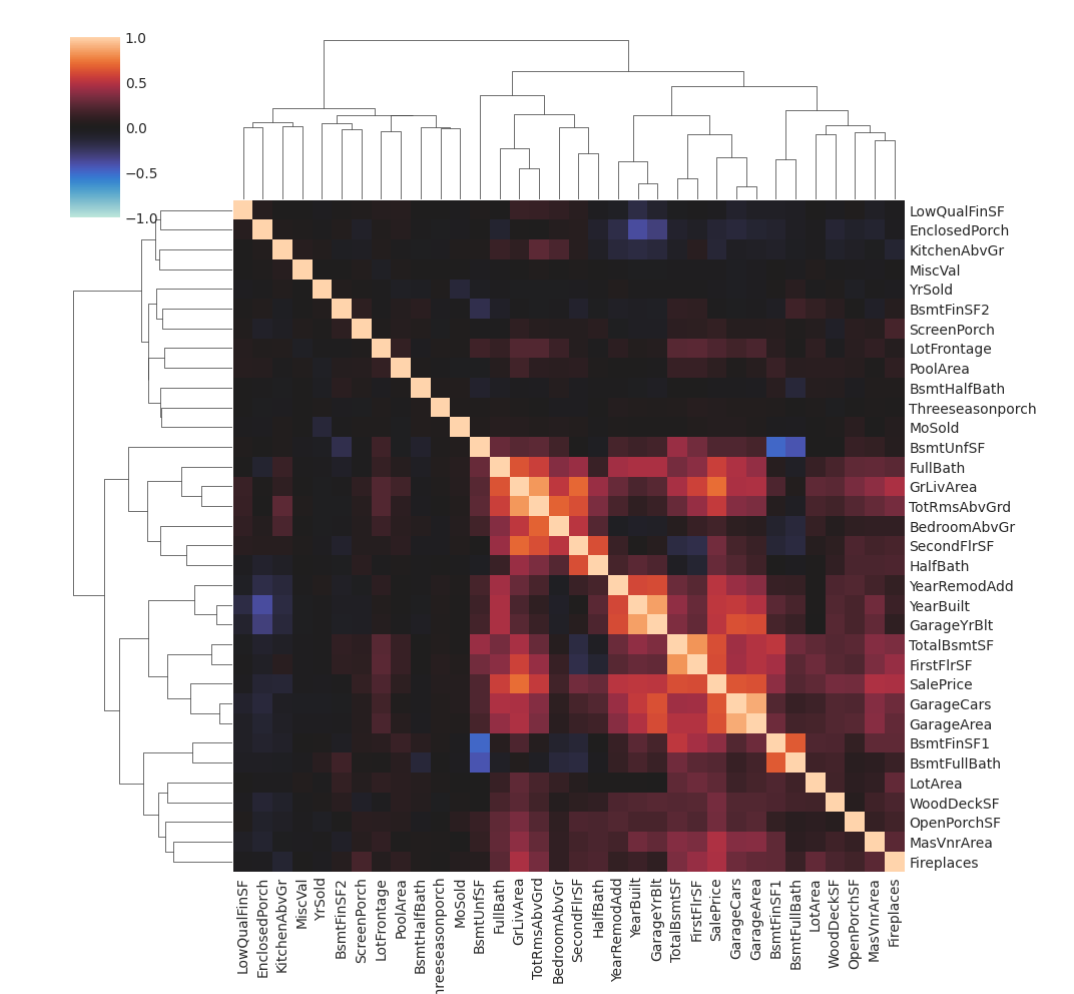
对于进一步分析，您可能想查看数据集的相关矩阵：

def corrplot(df, method="pearson", annot=True, **kwargs):
    sns.clustermap(
        df.corr(method, numeric_only=True),
        vmin=-1.0,
        vmax=1.0,
        cmap="icefire",
        method="complete",
        annot=annot,
        **kwargs,
    )

corrplot(df_train, annot=None)

高度相关特征组通常会产生有趣的载荷。

PCA应用 - 标识异常值

在练习5中，您应用PCA来确定数据中的异常值，即在其他数据中没有很好代表的房屋。您看到Edwards社区中有一组房屋，其SaleCondition为Partial，这些值特别极端。

一些模型可以从这些异常值的标识中受益，下一个转换就是这样做的。

def indicate_outliers(df):
    X_new = pd.DataFrame()
    X_new["Outlier"] = (df.Neighborhood == "Edwards") & (df.SaleCondition == "Partial")
    return X_new

目标编码

需要单独的保留集来创建目标编码是对数据的相当浪费。在教程6中，我们使用了25%的数据集仅仅为了编码一个特征Zipcode。那25%中其他特征的数据我们完全没有使用。

然而，有一种方法可以使用目标编码而不必使用保留编码数据。它基本上是交叉验证中使用的相同技巧：

将数据分成折叠，每个折叠有两个数据集分割。
在一个分割上训练编码器，但转换另一个分割的值。
对所有分割重复此过程。

这样，训练和转换总是在独立的数据集上进行，就像使用保留集一样，但不会浪费任何数据。

下面隐藏单元格中有一个可以与任何目标编码器一起使用的包装器：

class CrossFoldEncoder:
    def __init__(self, encoder, **kwargs):
        self.encoder_ = encoder
        self.kwargs_ = kwargs  # 编码器的关键字参数
        self.cv_ = KFold(n_splits=5)

    # 在一个分割上拟合编码器并转换另一个分割上的特征
    # 对所有折叠中的分割进行迭代，给出完整的
    # 转换。我们现在还有每个折叠上训练的一个编码器。
    def fit_transform(self, X, y, cols):
        self.fitted_encoders_ = []
        self.cols_ = cols
        X_encoded = []
        for idx_encode, idx_train in self.cv_.split(X):
            fitted_encoder = self.encoder_(cols=cols, **self.kwargs_)
            fitted_encoder.fit(
                X.iloc[idx_encode, :], y.iloc[idx_encode],
            )
            X_encoded.append(fitted_encoder.transform(X.iloc[idx_train, :])[cols])
            self.fitted_encoders_.append(fitted_encoder)
        X_encoded = pd.concat(X_encoded)
        X_encoded.columns = [name + "_encoded" for name in X_encoded.columns]
        return X_encoded
# 通过对从每个折叠学到的编码取平均值来转换测试数据
def transform(self, X):
    from functools import reduce

    X_encoded_list = []
    for fitted_encoder in self.fitted_encoders_:
        X_encoded = fitted_encoder.transform(X)
        X_encoded_list.append(X_encoded[self.cols_])
    X_encoded = reduce(
        lambda x, y: x.add(y, fill_value=0), X_encoded_list
    ) / len(X_encoded_list)
    X_encoded.columns = [name + "_encoded" for name in X_encoded.columns]
    return X_encoded

使用方法：

1 2	encoder = CrossFoldEncoder(MEstimateEncoder, m=1) X_encoded = encoder.fit_transform(X, y, cols=["MSSubClass"])

您可以将category_encoders库中的任何编码器转换为交叉折叠编码器。值得尝试CatBoostEncoder。它类似于MEstimateEncoder，但使用一些技巧来更好地防止过拟合。它的平滑参数被称为a而不是m。

创建最终特征集

现在让我们将所有内容组合在一起。将转换放在单独的函数中，使得实验各种组合更容易。我保留未注释的函数是我发现效果最好的。您应该尝试自己的想法！修改任何这些转换或提出一些您自己的转换来添加到管道中。

def create_features(df, df_test=None):
    X = df.copy()
    y = X.pop("SalePrice")
    mi_scores = make_mi_scores(X, y)

    # 如果提供了测试数据，则合并分割的数据集
    # 如果我们创建测试集预测的特征，我们应该使用我们可用的所有数据。
    # 创建特征后，我们将重新创建分割。
    if df_test is not None:
        X_test = df_test.copy()
        X_test.pop("SalePrice")
        X = pd.concat([X, X_test])

    # 第2课 - 互信息
    X = drop_uninformative(X, mi_scores)

    # 第3课 - 转换
    X = X.join(mathematical_transforms(X))
    X = X.join(interactions(X))
    X = X.join(counts(X))
    # X = X.join(break_down(X))
    X = X.join(group_transforms(X))

    # 第4课 - 聚类
    # X = X.join(cluster_labels(X, cluster_features, n_clusters=20))
    # X = X.join(cluster_distance(X, cluster_features, n_clusters=20))

    # 第5课 - PCA
    X = X.join(pca_inspired(X))
    # X = X.join(pca_components(X, pca_features))
    # X = X.join(indicate_outliers(X))

    X = label_encode(X)

    # 重新形成分割
    if df_test is not None:
        X_test = X.loc[df_test.index, :]
        X.drop(df_test.index, inplace=True)

    # 第6课 - 目标编码器
    encoder = CrossFoldEncoder(MEstimateEncoder, m=1)
    X = X.join(encoder.fit_transform(X, y, cols=["MSSubClass"]))
    if df_test is not None:
        X_test = X_test.join(encoder.transform(X_test))

    if df_test is not None:
        return X, X_test
    else:
        return X

df_train, df_test = load_data()
X_train = create_features(df_train)
y_train = df_train.loc[:, "SalePrice"]

score_dataset(X_train, y_train)

输出[23]:

1	0.13863986787521657

第四步 - 超参数调优

在这个阶段，您可能希望在创建最终提交之前对XGBoost进行一些超参数调优。

X_train = create_features(df_train)
y_train = df_train.loc[:, "SalePrice"]

xgb_params = dict(
    max_depth=6,         # 每棵树的最大深度 - 尝试2到10
    learning_rate=0.01,   # 每棵树的影响 - 尝试0.0001到0.1
    n_estimators=1000,    # 树的数量（即提升轮数）- 尝试1000到8000
    min_child_weight=1,   # 叶子节点中的最小房屋数 - 尝试1到10
    colsample_bytree=0.7, # 每棵树的特征（列）比例 - 尝试0.2到1.0
    subsample=0.7,        # 每棵树的实例（行）比例 - 尝试0.2到1.0
    reg_alpha=0.5,        # L1正则化（类似LASSO）- 尝试0.0到10.0
    reg_lambda=1.0,       # L2正则化（类似Ridge）- 尝试0.0到10.0
    num_parallel_tree=1,  # 设置 > 1 用于提升随机森林
)

xgb = XGBRegressor(**xgb_params)
score_dataset(X_train, y_train, xgb)

输出[24]:

1	0.12417177287599078

手动调整这些参数可以获得很好的结果。但是，您可能希望尝试使用scikit-learn的hyperparameter tuners。或者您可以探索更高级的调优库，如Optuna或scikit-optimize。

以下是如何使用Optuna和XGBoost：

import optuna

def objective(trial):
    xgb_params = dict(
        max_depth=trial.suggest_int("max_depth", 2, 10),
        learning_rate=trial.suggest_float("learning_rate", 1e-4, 1e-1, log=True),
        n_estimators=trial.suggest_int("n_estimators", 1000, 8000),
        min_child_weight=trial.suggest_int("min_child_weight", 1, 10),
        colsample_bytree=trial.suggest_float("colsample_bytree", 0.2, 1.0),
        subsample=trial.suggest_float("subsample", 0.2, 1.0),
        reg_alpha=trial.suggest_float("reg_alpha", 1e-4, 1e2, log=True),
        reg_lambda=trial.suggest_float("reg_lambda", 1e-4, 1e2, log=True),
    )
    xgb = XGBRegressor(**xgb_params)
    return score_dataset(X_train, y_train, xgb)

study = optuna.create_study(direction="minimize")
study.optimize(objective, n_trials=20)
xgb_params = study.best_params

将此代码复制到代码单元格中如果您想使用它，但请注意运行可能需要相当长的时间。完成后，您可能会喜欢使用Optuna的一些可视化工具。

第五步 - 训练模型并提交

一旦您对所有内容都满意，就可以创建最终预测了！这个单元将：

从原始数据创建特征集
在训练数据上训练XGBoost
使用训练好的模型从测试集生成预测
将预测保存到CSV文件

X_train, X_test = create_features(df_train, df_test)
y_train = df_train.loc[:, "SalePrice"]

xgb = XGBRegressor(**xgb_params)
# XGB最小化MSE，但竞赛损失是RMSLE
# 因此，我们需要对y进行对数变换来训练，并对预测进行指数变换
xgb.fit(X_train, np.log(y))
predictions = np.exp(xgb.predict(X_test))

output = pd.DataFrame({'Id': X_test.index, 'SalePrice': predictions})
output.to_csv('my_submission.csv', index=False)
print("Your submission was successfully saved!")